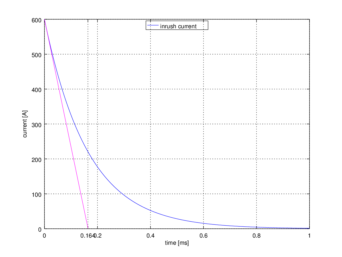
Featured image of post アンプの大容量平滑コンデンサの突入電流抑制回路

アンプの大容量平滑コンデンサの突入電流抑制回路

RC直列回路の回路方程式

コンデンサーに蓄えられる電荷を $q(t)$ として

$$ E = Ri(t) + \frac{q(t)}{C} \tag1 $$

$$ i(t) + \frac{dq(t)}{dt} \tag2 $$

(1), (2)式を $ q(0) = 0, \mathcal{L} q(t) = Q(s),\mathcal{L} i(t) = I(s) $ としてラプラス変換すると

$$ \frac{E}{s} = RI(s) + \frac{Q(s)}{C} \tag3 $$

$$ I(s) = sQ(s) $$

$$ Q(s) = \frac{I(s)}{s} \tag4 $$

(4)式を(3)式に代入して $$ \begin{aligned} \frac{E}{s} &= RI(s) + \frac{I(s)}{sC} \\[1em] \frac{E}{s} &= \Bigl( R + \frac{1}{sC} \Bigr) I(s){\Huge } \tag5 \end{aligned} $$

(5)式より電流 $ I(s) $ は

$$ \begin{aligned} I(s) &= \frac{E}{s} \cdot \Biggl( \frac{1}{R + \frac{1}{sC} }\Biggr) \\[1em] I(s) &= \frac{E}{s} \cdot \frac{1}{R} \Biggl( \frac{1}{1 + \frac{1}{sRC} } \Biggr) \\[1em] I(s) &= \frac{E}{R} \cdot \frac{1}{s} \Biggl( \frac{1}{1 + \frac{1}{sRC} } \Biggr) \\[1em] I(s) &= \frac{E}{R} \cdot \Biggl( \frac{1}{s + \frac{1}{RC} } \Biggr) \tag{6} \end{aligned} $$

ここでラプラス変換の公式

$ f(t) = e^{-at} \Longleftrightarrow F(s) = \frac{1}{s+a} $

(6)式を逆ラプラス変換して

$$ \Large i(t) = \frac{E}{R} e ^ {- \frac{1}{RC} t} \tag7 $$

コンデンサーに流れる電流の式が得られた.

突入電流を抑制しない場合にコンデンサーに流れる電流

RC直列回路

  • E = 12V
  • R = ESR = 0.020Ω
  • C = 8200uF

の時

$$ \Large i(t) = \frac{12}{0.020} e ^ {- \frac{1}{0.020~\cdot~0.0082} t} $$

時定数 $ \tau $ (初期の変化率を維持した時にx軸と交差する点)
$$ \tau = RC = 0.020 \cdot 0.0082 = 0.164ms $$

最大突入電流(t=0の電流) $$ I_{peak} = \frac{12}{0.020} = 600A $$

突入電流と初期の変化率を維持した時のグラフ

 1
 2
 3
 4
 5
 6
 7
 8
 9
10
11
12
13
14
15
16
17
18
19
20
21
22
23
24
25
26
27
28
29
30
31
32
33
34
%
% 突入電流を計算する
% https://ak1211.com
% Copyright (c) 2015 Akihiro Yamamoto
%
%
% This software is released under the MIT License.
% http://opensource.org/licenses/mit-license.php
%
e = 12;
r = 0.020;
c = 0.0082;

t = linspace(0, 0.001, 1000);
i = e / r * exp(-1/(r*c)*t);


plot(t*1000, i, 'cb-');
grid on;
hold on;

xticks = get(gca(), "xtick");
xticks = [xticks  [0.164]  ];
xticks = sort(xticks);
set(gca(), "xtick", xticks);

xlabel ('time [ms]');
ylabel ('current [A]');
legend ('inrush current', "location", 'north');

d = (i(2)-i(1))/(t(2)-t(1));
y = i(1) + d*t;
y(y<0.0) = NA;
plot(t*1000, y, 'cm-');

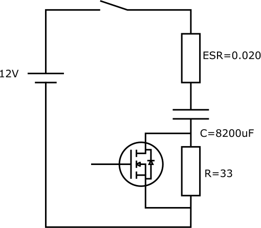
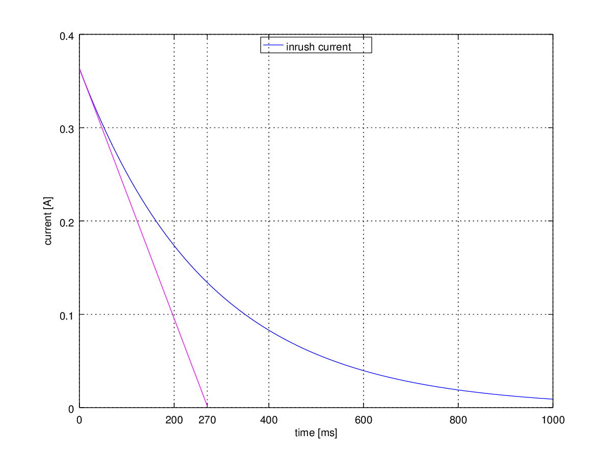
突入電流を抑制した場合にコンデンサーに流れる電流
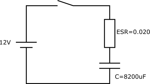
突入電流抑制回路

  • E = 12V
  • R = 33 + ESR = 33.020Ω
  • C = 8200uF

の時 $$ \Large i(t) = \frac{12}{33.020} e ^ {- \frac{1}{33.020~\cdot~0.0082} t} $$

時定数 $ \tau $ $$ \tau = RC = 33.020 \cdot 0.0082 = 270.76ms $$

最大突入電流(t=0の電流) $$ I_{peak} = \frac{12}{33.020} = 363.42mA $$

突入電流抑制時と初期の変化率を維持した時のグラフ

 1
 2
 3
 4
 5
 6
 7
 8
 9
10
11
12
13
14
15
16
17
18
19
20
21
22
23
24
25
26
27
28
29
30
31
32
33
34
%
% 突入電流を計算する
% http://ak1211.com
% Copyright (c) 2015 Akihiro Yamamoto
%
%
% This software is released under the MIT License.
% http://opensource.org/licenses/mit-license.php
%
e = 12;
r = 33+0.020;
c = 0.0082;

t = linspace(0, 1, 1000);
i = e / r * exp(-1/(r*c)*t);


plot(t*1000, i, 'cb-');
grid on;
hold on;

xticks = get(gca(), "xtick");
xticks = [xticks  [270]  ];
xticks = sort(xticks);
set(gca(), "xtick", xticks);

xlabel ('time [ms]');
ylabel ('current [A]');
legend ('inrush current', "location", 'north');

d = (i(2)-i(1))/(t(2)-t(1));
y = i(1) + d*t;
y(y<0.0) = NA;
plot(t*1000, y, 'cm-');

作った突入電流抑制回路

突入電流抑制回路

  1. 突入電流抑制中はMOSFETはOFFであって, 抵抗で突入電流を抑制
  2. 一定時間後にMCUによってMOSFETをONにして抵抗をバイパスします。
comments powered by Disqus

This website uses cookies to improve your experience.
このサイトは「Googleアナリティクス」を使用しています。
Googleアナリティクスはデータの収集のためにCookieを使用しています。


Built with Hugo
テーマ StackJimmy によって設計されています。